Training Custom Object Detector
So, up to now you should have done the following:
Installed TensorFlow (See TensorFlow Installation)
Installed TensorFlow Object Detection API (See TensorFlow Object Detection API Installation)
Now that we have done all the above, we can start doing some cool stuff. Here we will see how you can train your own object detector, and since it is not as simple as it sounds, we will have a look at:
How to organise your workspace/training files
How to prepare/annotate image datasets
How to generate tf records from such datasets
How to configure a simple training pipeline
How to train a model and monitor it’s progress
How to export the resulting model and use it to detect objects.
Preparing the Workspace
If you have followed the tutorial, you should by now have a folder
Tensorflow, placed under<PATH_TO_TF>(e.g.C:/Users/sglvladi/Documents), with the following directory tree:TensorFlow/ ├─ addons/ (Optional) │ └─ labelImg/ └─ models/ ├─ community/ ├─ official/ ├─ orbit/ ├─ research/ └─ ...
Now create a new folder under
TensorFlowand call itworkspace. It is within theworkspacethat we will store all our training set-ups. Now let’s go under workspace and create another folder namedtraining_demo. Now our directory structure should be as so:TensorFlow/ ├─ addons/ (Optional) │ └─ labelImg/ ├─ models/ │ ├─ community/ │ ├─ official/ │ ├─ orbit/ │ ├─ research/ │ └─ ... └─ workspace/ └─ training_demo/
The
training_demofolder shall be our training folder, which will contain all files related to our model training. It is advisable to create a separate training folder each time we wish to train on a different dataset. The typical structure for training folders is shown below.training_demo/ ├─ annotations/ ├─ exported-models/ ├─ images/ │ ├─ test/ │ └─ train/ ├─ models/ ├─ pre-trained-models/ └─ README.md
Here’s an explanation for each of the folders/filer shown in the above tree:
annotations: This folder will be used to store all*.csvfiles and the respective TensorFlow*.recordfiles, which contain the list of annotations for our dataset images.exported-models: This folder will be used to store exported versions of our trained model(s).images: This folder contains a copy of all the images in our dataset, as well as the respective*.xmlfiles produced for each one, oncelabelImgis used to annotate objects.images/train: This folder contains a copy of all images, and the respective*.xmlfiles, which will be used to train our model.images/test: This folder contains a copy of all images, and the respective*.xmlfiles, which will be used to test our model.
models: This folder will contain a sub-folder for each of training job. Each subfolder will contain the training pipeline configuration file*.config, as well as all files generated during the training and evaluation of our model.pre-trained-models: This folder will contain the downloaded pre-trained models, which shall be used as a starting checkpoint for our training jobs.README.md: This is an optional file which provides some general information regarding the training conditions of our model. It is not used by TensorFlow in any way, but it generally helps when you have a few training folders and/or you are revisiting a trained model after some time.
If you do not understand most of the things mentioned above, no need to worry, as we’ll see how all the files are generated further down.
Preparing the Dataset
Annotate the Dataset
Install LabelImg
There exist several ways to install labelImg. Below are 3 of the most common.
Using PIP (Recommended)
Open a new Terminal window and activate the tensorflow_gpu environment (if you have not done so already)
Run the following command to install
labelImg:
pip install labelImg
labelImgcan then be run as follows:
labelImg
# or
labelImg [IMAGE_PATH] [PRE-DEFINED CLASS FILE]
Use precompiled binaries (Easy)
Precompiled binaries for both Windows and Linux can be found here .
Installation is the done in three simple steps:
Inside you
TensorFlowfolder, create a new directory, name itaddonsand thencdinto it.Download the latest binary for your OS from here. and extract its contents under
Tensorflow/addons/labelImg.You should now have a single folder named
addons/labelImgunder yourTensorFlowfolder, which contains another 4 folders as such:
TensorFlow/
├─ addons/
│  └─ labelImg/
└─ models/
   ├─ community/
   ├─ official/
   ├─ orbit/
   ├─ research/
   └─ ...
labelImgcan then be run as follows:
# From within Tensorflow/addons/labelImg
labelImg
# or
labelImg [IMAGE_PATH] [PRE-DEFINED CLASS FILE]
Build from source (Hard)
The steps for installing from source follow below.
1. Download labelImg
Inside you
TensorFlowfolder, create a new directory, name itaddonsand thencdinto it.To download the package you can either use Git to clone the labelImg repo inside the
TensorFlow\addonsfolder, or you can simply download it as a ZIP and extract it’s contents inside theTensorFlow\addonsfolder. To keep things consistent, in the latter case you will have to rename the extracted folderlabelImg-mastertolabelImg. [1]You should now have a single folder named
addons\labelImgunder yourTensorFlowfolder, which contains another 4 folders as such:
TensorFlow/
├─ addons
│  └─ labelImg/
└─ models/
   ├─ community/
   ├─ official/
   ├─ orbit/
   ├─ research/
   └─ ...
2. Install dependencies and compiling package
Open a new Terminal window and activate the tensorflow_gpu environment (if you have not done so already)
cdintoTensorFlow/addons/labelImgand run the following commands:conda install pyqt=5 pyrcc5 -o libs/resources.py resources.qrc
sudo apt-get install pyqt5-dev-tools
sudo pip install -r requirements/requirements-linux-python3.txt
make qt5py3
3. Test your installation
Open a new Terminal window and activate the tensorflow_gpu environment (if you have not done so already)
cdintoTensorFlow/addons/labelImgand run the following command:# From within Tensorflow/addons/labelImg python labelImg.py # or python labelImg.py [IMAGE_PATH] [PRE-DEFINED CLASS FILE]
Annotate Images
Once you have collected all the images to be used to test your model (ideally more than 100 per class), place them inside the folder
training_demo/images.Open a new Terminal window.
Next go ahead and start
labelImg, pointing it to yourtraining_demo/imagesfolder.If you installed
labelImgUsing PIP (Recommended):
labelImg <PATH_TO_TF>/TensorFlow/workspace/training_demo/images
Othewise,
cdintoTensorflow/addons/labelImgand run:
# From within Tensorflow/addons/labelImg
python labelImg.py ../../workspace/training_demo/images
A File Explorer Dialog windows should open, which points to the
training_demo/imagesfolder.Press the “Select Folder” button, to start annotating your images.
Once open, you should see a window similar to the one below:
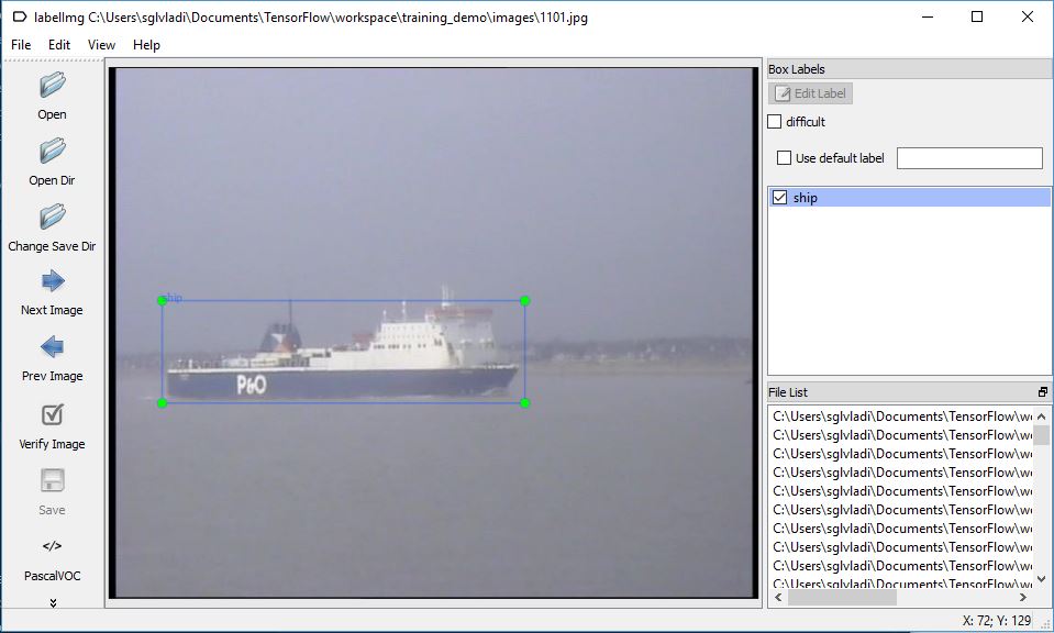
I won’t be covering a tutorial on how to use labelImg, but you can have a look at labelImg’s repo for more details. A nice Youtube video demonstrating how to use labelImg is also available here. What is important is that once you annotate all your images, a set of new *.xml files, one for each image, should be generated inside your training_demo/images folder.
Partition the Dataset
Once you have finished annotating your image dataset, it is a general convention to use only part of it for training, and the rest is used for evaluation purposes (e.g. as discussed in Evaluating the Model (Optional)).
Typically, the ratio is 9:1, i.e. 90% of the images are used for training and the rest 10% is maintained for testing, but you can chose whatever ratio suits your needs.
Once you have decided how you will be splitting your dataset, copy all training images, together
with their corresponding *.xml files, and place them inside the training_demo/images/train
folder. Similarly, copy all testing images, with their *.xml files, and paste them inside
training_demo/images/test.
For lazy people like myself, who cannot be bothered to do the above, I have put together a simple script that automates the above process:
""" usage: partition_dataset.py [-h] [-i IMAGEDIR] [-o OUTPUTDIR] [-r RATIO] [-x]

Partition dataset of images into training and testing sets

optional arguments:
  -h, --help            show this help message and exit
  -i IMAGEDIR, --imageDir IMAGEDIR
                        Path to the folder where the image dataset is stored. If not specified, the CWD will be used.
  -o OUTPUTDIR, --outputDir OUTPUTDIR
                        Path to the output folder where the train and test dirs should be created. Defaults to the same directory as IMAGEDIR.
  -r RATIO, --ratio RATIO
                        The ratio of the number of test images over the total number of images. The default is 0.1.
  -x, --xml             Set this flag if you want the xml annotation files to be processed and copied over.
"""
import os
import re
from shutil import copyfile
import argparse
import math
import random


def iterate_dir(source, dest, ratio, copy_xml):
    source = source.replace('\\', '/')
    dest = dest.replace('\\', '/')
    train_dir = os.path.join(dest, 'train')
    test_dir = os.path.join(dest, 'test')

    if not os.path.exists(train_dir):
        os.makedirs(train_dir)
    if not os.path.exists(test_dir):
        os.makedirs(test_dir)

    images = [f for f in os.listdir(source)
              if re.search(r'([a-zA-Z0-9\s_\\.\-\(\):])+(?i)(.jpg|.jpeg|.png)$', f)]

    num_images = len(images)
    num_test_images = math.ceil(ratio*num_images)

    for i in range(num_test_images):
        idx = random.randint(0, len(images)-1)
        filename = images[idx]
        copyfile(os.path.join(source, filename),
                 os.path.join(test_dir, filename))
        if copy_xml:
            xml_filename = os.path.splitext(filename)[0]+'.xml'
            copyfile(os.path.join(source, xml_filename),
                     os.path.join(test_dir,xml_filename))
        images.remove(images[idx])

    for filename in images:
        copyfile(os.path.join(source, filename),
                 os.path.join(train_dir, filename))
        if copy_xml:
            xml_filename = os.path.splitext(filename)[0]+'.xml'
            copyfile(os.path.join(source, xml_filename),
                     os.path.join(train_dir, xml_filename))


def main():

    # Initiate argument parser
    parser = argparse.ArgumentParser(description="Partition dataset of images into training and testing sets",
                                     formatter_class=argparse.RawTextHelpFormatter)
    parser.add_argument(
        '-i', '--imageDir',
        help='Path to the folder where the image dataset is stored. If not specified, the CWD will be used.',
        type=str,
        default=os.getcwd()
    )
    parser.add_argument(
        '-o', '--outputDir',
        help='Path to the output folder where the train and test dirs should be created. '
             'Defaults to the same directory as IMAGEDIR.',
        type=str,
        default=None
    )
    parser.add_argument(
        '-r', '--ratio',
        help='The ratio of the number of test images over the total number of images. The default is 0.1.',
        default=0.1,
        type=float)
    parser.add_argument(
        '-x', '--xml',
        help='Set this flag if you want the xml annotation files to be processed and copied over.',
        action='store_true'
    )
    args = parser.parse_args()

    if args.outputDir is None:
        args.outputDir = args.imageDir

    # Now we are ready to start the iteration
    iterate_dir(args.imageDir, args.outputDir, args.ratio, args.xml)


if __name__ == '__main__':
    main()
Under the
TensorFlowfolder, create a new folderTensorFlow/scripts, which we can use to store some useful scripts.To make things even tidier, let’s create a new folder
TensorFlow/scripts/preprocessing, where we shall store scripts that we can use to preprocess our training inputs. Below is outTensorFlowdirectory tree structure, up to now:TensorFlow/ ├─ addons/ (Optional) │ └─ labelImg/ ├─ models/ │ ├─ community/ │ ├─ official/ │ ├─ orbit/ │ ├─ research/ │ └─ ... ├─ scripts/ │ └─ preprocessing/ └─ workspace/ └─ training_demo/
Click
hereto download the above script and save it insideTensorFlow/scripts/preprocessing.Then,
cdintoTensorFlow/scripts/preprocessingand run:python partition_dataset.py -x -i [PATH_TO_IMAGES_FOLDER] -r 0.1 # For example # python partition_dataset.py -x -i C:/Users/sglvladi/Documents/Tensorflow/workspace/training_demo/images -r 0.1
Once the script has finished, two new folders should have been created under training_demo/images,
namely training_demo/images/train and training_demo/images/test, containing 90% and 10% of
the images (and *.xml files), respectively. To avoid loss of any files, the script will not
delete the images under training_demo/images. Once you have checked that your images have been
safely copied over, you can delete the images under training_demo/images manually.
Create Label Map
TensorFlow requires a label map, which namely maps each of the used labels to an integer values. This label map is used both by the training and detection processes.
Below we show an example label map (e.g label_map.pbtxt), assuming that our dataset contains 2 labels, dogs and cats:
item {
    id: 1
    name: 'cat'
}

item {
    id: 2
    name: 'dog'
}
Label map files have the extention .pbtxt and should be placed inside the training_demo/annotations folder.
Create TensorFlow Records
Now that we have generated our annotations and split our dataset into the desired training and
testing subsets, it is time to convert our annotations into the so called TFRecord format.
Convert *.xml to *.record
To do this we can write a simple script that iterates through all *.xml files in the
training_demo/images/train and training_demo/images/test folders, and generates a
*.record file for each of the two. Here is an example script that allows us to do just that:
""" Sample TensorFlow XML-to-TFRecord converter

usage: generate_tfrecord.py [-h] [-x XML_DIR] [-l LABELS_PATH] [-o OUTPUT_PATH] [-i IMAGE_DIR] [-c CSV_PATH]

optional arguments:
  -h, --help            show this help message and exit
  -x XML_DIR, --xml_dir XML_DIR
                        Path to the folder where the input .xml files are stored.
  -l LABELS_PATH, --labels_path LABELS_PATH
                        Path to the labels (.pbtxt) file.
  -o OUTPUT_PATH, --output_path OUTPUT_PATH
                        Path of output TFRecord (.record) file.
  -i IMAGE_DIR, --image_dir IMAGE_DIR
                        Path to the folder where the input image files are stored. Defaults to the same directory as XML_DIR.
  -c CSV_PATH, --csv_path CSV_PATH
                        Path of output .csv file. If none provided, then no file will be written.
"""

import os
import glob
import pandas as pd
import io
import xml.etree.ElementTree as ET
import argparse

os.environ['TF_CPP_MIN_LOG_LEVEL'] = '2'    # Suppress TensorFlow logging (1)
import tensorflow.compat.v1 as tf
from PIL import Image
from object_detection.utils import dataset_util, label_map_util
from collections import namedtuple

# Initiate argument parser
parser = argparse.ArgumentParser(
    description="Sample TensorFlow XML-to-TFRecord converter")
parser.add_argument("-x",
                    "--xml_dir",
                    help="Path to the folder where the input .xml files are stored.",
                    type=str)
parser.add_argument("-l",
                    "--labels_path",
                    help="Path to the labels (.pbtxt) file.", type=str)
parser.add_argument("-o",
                    "--output_path",
                    help="Path of output TFRecord (.record) file.", type=str)
parser.add_argument("-i",
                    "--image_dir",
                    help="Path to the folder where the input image files are stored. "
                         "Defaults to the same directory as XML_DIR.",
                    type=str, default=None)
parser.add_argument("-c",
                    "--csv_path",
                    help="Path of output .csv file. If none provided, then no file will be "
                         "written.",
                    type=str, default=None)

args = parser.parse_args()

if args.image_dir is None:
    args.image_dir = args.xml_dir

label_map = label_map_util.load_labelmap(args.labels_path)
label_map_dict = label_map_util.get_label_map_dict(label_map)


def xml_to_csv(path):
    """Iterates through all .xml files (generated by labelImg) in a given directory and combines
    them in a single Pandas dataframe.

    Parameters:
    ----------
    path : str
        The path containing the .xml files
    Returns
    -------
    Pandas DataFrame
        The produced dataframe
    """

    xml_list = []
    for xml_file in glob.glob(path + '/*.xml'):
        tree = ET.parse(xml_file)
        root = tree.getroot()
        filename = root.find('filename').text
        width = int(root.find('size').find('width').text)
        height = int(root.find('size').find('height').text)
        for member in root.findall('object'):
            bndbox = member.find('bndbox')
            value = (filename,
                     width,
                     height,
                     member.find('name').text,
                     int(bndbox.find('xmin').text),
                     int(bndbox.find('ymin').text),
                     int(bndbox.find('xmax').text),
                     int(bndbox.find('ymax').text),
                     )
            xml_list.append(value)
    column_name = ['filename', 'width', 'height',
                   'class', 'xmin', 'ymin', 'xmax', 'ymax']
    xml_df = pd.DataFrame(xml_list, columns=column_name)
    return xml_df


def class_text_to_int(row_label):
    return label_map_dict[row_label]


def split(df, group):
    data = namedtuple('data', ['filename', 'object'])
    gb = df.groupby(group)
    return [data(filename, gb.get_group(x)) for filename, x in zip(gb.groups.keys(), gb.groups)]


def create_tf_example(group, path):
    with tf.gfile.GFile(os.path.join(path, '{}'.format(group.filename)), 'rb') as fid:
        encoded_jpg = fid.read()
    encoded_jpg_io = io.BytesIO(encoded_jpg)
    image = Image.open(encoded_jpg_io)
    width, height = image.size

    filename = group.filename.encode('utf8')
    image_format = b'jpg'
    xmins = []
    xmaxs = []
    ymins = []
    ymaxs = []
    classes_text = []
    classes = []

    for index, row in group.object.iterrows():
        xmins.append(row['xmin'] / width)
        xmaxs.append(row['xmax'] / width)
        ymins.append(row['ymin'] / height)
        ymaxs.append(row['ymax'] / height)
        classes_text.append(row['class'].encode('utf8'))
        classes.append(class_text_to_int(row['class']))

    tf_example = tf.train.Example(features=tf.train.Features(feature={
        'image/height': dataset_util.int64_feature(height),
        'image/width': dataset_util.int64_feature(width),
        'image/filename': dataset_util.bytes_feature(filename),
        'image/source_id': dataset_util.bytes_feature(filename),
        'image/encoded': dataset_util.bytes_feature(encoded_jpg),
        'image/format': dataset_util.bytes_feature(image_format),
        'image/object/bbox/xmin': dataset_util.float_list_feature(xmins),
        'image/object/bbox/xmax': dataset_util.float_list_feature(xmaxs),
        'image/object/bbox/ymin': dataset_util.float_list_feature(ymins),
        'image/object/bbox/ymax': dataset_util.float_list_feature(ymaxs),
        'image/object/class/text': dataset_util.bytes_list_feature(classes_text),
        'image/object/class/label': dataset_util.int64_list_feature(classes),
    }))
    return tf_example


def main(_):

    writer = tf.python_io.TFRecordWriter(args.output_path)
    path = os.path.join(args.image_dir)
    examples = xml_to_csv(args.xml_dir)
    grouped = split(examples, 'filename')
    for group in grouped:
        tf_example = create_tf_example(group, path)
        writer.write(tf_example.SerializeToString())
    writer.close()
    print('Successfully created the TFRecord file: {}'.format(args.output_path))
    if args.csv_path is not None:
        examples.to_csv(args.csv_path, index=None)
        print('Successfully created the CSV file: {}'.format(args.csv_path))


if __name__ == '__main__':
    tf.app.run()
Click
hereto download the above script and save it insideTensorFlow/scripts/preprocessing.Install the
pandaspackage:conda install pandas # Anaconda # or pip install pandas # pip
Finally,
cdintoTensorFlow/scripts/preprocessingand run:# Create train data: python generate_tfrecord.py -x [PATH_TO_IMAGES_FOLDER]/train -l [PATH_TO_ANNOTATIONS_FOLDER]/label_map.pbtxt -o [PATH_TO_ANNOTATIONS_FOLDER]/train.record # Create test data: python generate_tfrecord.py -x [PATH_TO_IMAGES_FOLDER]/test -l [PATH_TO_ANNOTATIONS_FOLDER]/label_map.pbtxt -o [PATH_TO_ANNOTATIONS_FOLDER]/test.record # For example # python generate_tfrecord.py -x C:/Users/sglvladi/Documents/Tensorflow/workspace/training_demo/images/train -l C:/Users/sglvladi/Documents/Tensorflow/workspace/training_demo/annotations/label_map.pbtxt -o C:/Users/sglvladi/Documents/Tensorflow/workspace/training_demo/annotations/train.record # python generate_tfrecord.py -x C:/Users/sglvladi/Documents/Tensorflow/workspace/training_demo/images/test -l C:/Users/sglvladi/Documents/Tensorflow2/workspace/training_demo/annotations/label_map.pbtxt -o C:/Users/sglvladi/Documents/Tensorflow/workspace/training_demo/annotations/test.record
Once the above is done, there should be 2 new files under the training_demo/annotations folder, named test.record and train.record, respectively.
Configuring a Training Job
For the purposes of this tutorial we will not be creating a training job from scratch, but rather we will reuse one of the pre-trained models provided by TensorFlow. If you would like to train an entirely new model, you can have a look at TensorFlow’s tutorial.
The model we shall be using in our examples is the SSD ResNet50 V1 FPN 640x640 model, since it provides a relatively good trade-off between performance and speed. However, there exist a number of other models you can use, all of which are listed in TensorFlow 2 Detection Model Zoo.
Download Pre-Trained Model
To begin with, we need to download the latest pre-trained network for the model we wish to use.
This can be done by simply clicking on the name of the desired model in the table found in
TensorFlow 2 Detection Model Zoo.
Clicking on the name of your model should initiate a download for a *.tar.gz file.
Once the *.tar.gz file has been downloaded, open it using a decompression program of your
choice (e.g. 7zip, WinZIP, etc.). Next, open the *.tar folder that you see when the compressed
folder is opened, and extract its contents inside the folder training_demo/pre-trained-models.
Since we downloaded the SSD ResNet50 V1 FPN 640x640
model, our training_demo directory should now look as follows:
training_demo/
├─ ...
├─ pre-trained-models/
│  └─ ssd_resnet50_v1_fpn_640x640_coco17_tpu-8/
│     ├─ checkpoint/
│     ├─ saved_model/
│     └─ pipeline.config
└─ ...
Note that the above process can be repeated for all other pre-trained models you wish to experiment with. For example, if you wanted to also configure a training job for the EfficientDet D1 640x640 model, you can download the model and after extracting its context the demo directory will be:
training_demo/
├─ ...
├─ pre-trained-models/
│  ├─ efficientdet_d1_coco17_tpu-32/
│  │  ├─ checkpoint/
│  │  ├─ saved_model/
│  │  └─ pipeline.config
│  └─ ssd_resnet50_v1_fpn_640x640_coco17_tpu-8/
│     ├─ checkpoint/
│     ├─ saved_model/
│     └─ pipeline.config
└─ ...
Configure the Training Pipeline
Now that we have downloaded and extracted our pre-trained model, let’s create a directory for our
training job. Under the training_demo/models create a new directory named my_ssd_resnet50_v1_fpn
and copy the training_demo/pre-trained-models/ssd_resnet50_v1_fpn_640x640_coco17_tpu-8/pipeline.config
file inside the newly created directory. Our training_demo/models directory should now look
like this:
training_demo/
├─ ...
├─ models/
│  └─ my_ssd_resnet50_v1_fpn/
│     └─ pipeline.config
└─ ...
Now, let’s have a look at the changes that we shall need to apply to the pipeline.config file
(highlighted in yellow):
  1model {
  2  ssd {
  3    num_classes: 1 # Set this to the number of different label classes
  4    image_resizer {
  5      fixed_shape_resizer {
  6        height: 640
  7        width: 640
  8      }
  9    }
 10    feature_extractor {
 11      type: "ssd_resnet50_v1_fpn_keras"
 12      depth_multiplier: 1.0
 13      min_depth: 16
 14      conv_hyperparams {
 15        regularizer {
 16          l2_regularizer {
 17            weight: 0.00039999998989515007
 18          }
 19        }
 20        initializer {
 21          truncated_normal_initializer {
 22            mean: 0.0
 23            stddev: 0.029999999329447746
 24          }
 25        }
 26        activation: RELU_6
 27        batch_norm {
 28          decay: 0.996999979019165
 29          scale: true
 30          epsilon: 0.0010000000474974513
 31        }
 32      }
 33      override_base_feature_extractor_hyperparams: true
 34      fpn {
 35        min_level: 3
 36        max_level: 7
 37      }
 38    }
 39    box_coder {
 40      faster_rcnn_box_coder {
 41        y_scale: 10.0
 42        x_scale: 10.0
 43        height_scale: 5.0
 44        width_scale: 5.0
 45      }
 46    }
 47    matcher {
 48      argmax_matcher {
 49        matched_threshold: 0.5
 50        unmatched_threshold: 0.5
 51        ignore_thresholds: false
 52        negatives_lower_than_unmatched: true
 53        force_match_for_each_row: true
 54        use_matmul_gather: true
 55      }
 56    }
 57    similarity_calculator {
 58      iou_similarity {
 59      }
 60    }
 61    box_predictor {
 62      weight_shared_convolutional_box_predictor {
 63        conv_hyperparams {
 64          regularizer {
 65            l2_regularizer {
 66              weight: 0.00039999998989515007
 67            }
 68          }
 69          initializer {
 70            random_normal_initializer {
 71              mean: 0.0
 72              stddev: 0.009999999776482582
 73            }
 74          }
 75          activation: RELU_6
 76          batch_norm {
 77            decay: 0.996999979019165
 78            scale: true
 79            epsilon: 0.0010000000474974513
 80          }
 81        }
 82        depth: 256
 83        num_layers_before_predictor: 4
 84        kernel_size: 3
 85        class_prediction_bias_init: -4.599999904632568
 86      }
 87    }
 88    anchor_generator {
 89      multiscale_anchor_generator {
 90        min_level: 3
 91        max_level: 7
 92        anchor_scale: 4.0
 93        aspect_ratios: 1.0
 94        aspect_ratios: 2.0
 95        aspect_ratios: 0.5
 96        scales_per_octave: 2
 97      }
 98    }
 99    post_processing {
100      batch_non_max_suppression {
101        score_threshold: 9.99999993922529e-09
102        iou_threshold: 0.6000000238418579
103        max_detections_per_class: 100
104        max_total_detections: 100
105        use_static_shapes: false
106      }
107      score_converter: SIGMOID
108    }
109    normalize_loss_by_num_matches: true
110    loss {
111      localization_loss {
112        weighted_smooth_l1 {
113        }
114      }
115      classification_loss {
116        weighted_sigmoid_focal {
117          gamma: 2.0
118          alpha: 0.25
119        }
120      }
121      classification_weight: 1.0
122      localization_weight: 1.0
123    }
124    encode_background_as_zeros: true
125    normalize_loc_loss_by_codesize: true
126    inplace_batchnorm_update: true
127    freeze_batchnorm: false
128  }
129}
130train_config {
131  batch_size: 8 # Increase/Decrease this value depending on the available memory (Higher values require more memory and vice-versa)
132  data_augmentation_options {
133    random_horizontal_flip {
134    }
135  }
136  data_augmentation_options {
137    random_crop_image {
138      min_object_covered: 0.0
139      min_aspect_ratio: 0.75
140      max_aspect_ratio: 3.0
141      min_area: 0.75
142      max_area: 1.0
143      overlap_thresh: 0.0
144    }
145  }
146  sync_replicas: true
147  optimizer {
148    momentum_optimizer {
149      learning_rate {
150        cosine_decay_learning_rate {
151          learning_rate_base: 0.03999999910593033
152          total_steps: 25000
153          warmup_learning_rate: 0.013333000242710114
154          warmup_steps: 2000
155        }
156      }
157      momentum_optimizer_value: 0.8999999761581421
158    }
159    use_moving_average: false
160  }
161  fine_tune_checkpoint: "pre-trained-models/ssd_resnet50_v1_fpn_640x640_coco17_tpu-8/checkpoint/ckpt-0" # Path to checkpoint of pre-trained model
162  num_steps: 25000
163  startup_delay_steps: 0.0
164  replicas_to_aggregate: 8
165  max_number_of_boxes: 100
166  unpad_groundtruth_tensors: false
167  fine_tune_checkpoint_type: "detection" # Set this to "detection" since we want to be training the full detection model
168  use_bfloat16: false # Set this to false if you are not training on a TPU
169  fine_tune_checkpoint_version: V2
170}
171train_input_reader {
172  label_map_path: "annotations/label_map.pbtxt" # Path to label map file
173  tf_record_input_reader {
174    input_path: "annotations/train.record" # Path to training TFRecord file
175  }
176}
177eval_config {
178  metrics_set: "coco_detection_metrics"
179  use_moving_averages: false
180}
181eval_input_reader {
182  label_map_path: "annotations/label_map.pbtxt" # Path to label map file
183  shuffle: false
184  num_epochs: 1
185  tf_record_input_reader {
186    input_path: "annotations/test.record" # Path to testing TFRecord
187  }
188}
It is worth noting here that the changes to lines 178 to 179 above are optional. These
should only be used if you installed the COCO evaluation tools, as outlined in the
COCO API installation section, and you intend to run evaluation (see Evaluating the Model (Optional)).
Once the above changes have been applied to our config file, go ahead and save it.
Training the Model
Before we begin training our model, let’s go and copy the TensorFlow/models/research/object_detection/model_main_tf2.py
script and paste it straight into our training_demo folder. We will need this script in order
to train our model.
Now, to initiate a new training job, open a new Terminal, cd inside the training_demo
folder and run the following command:
python model_main_tf2.py --model_dir=models/my_ssd_resnet50_v1_fpn --pipeline_config_path=models/my_ssd_resnet50_v1_fpn/pipeline.config
Once the training process has been initiated, you should see a series of print outs similar to the one below (plus/minus some warnings):
...
WARNING:tensorflow:Unresolved object in checkpoint: (root).model._box_predictor._base_tower_layers_for_heads.class_predictions_with_background.4.10.gamma
W0716 05:24:19.105542  1364 util.py:143] Unresolved object in checkpoint: (root).model._box_predictor._base_tower_layers_for_heads.class_predictions_with_background.4.10.gamma
WARNING:tensorflow:Unresolved object in checkpoint: (root).model._box_predictor._base_tower_layers_for_heads.class_predictions_with_background.4.10.beta
W0716 05:24:19.106541  1364 util.py:143] Unresolved object in checkpoint: (root).model._box_predictor._base_tower_layers_for_heads.class_predictions_with_background.4.10.beta
WARNING:tensorflow:Unresolved object in checkpoint: (root).model._box_predictor._base_tower_layers_for_heads.class_predictions_with_background.4.10.moving_mean
W0716 05:24:19.107540  1364 util.py:143] Unresolved object in checkpoint: (root).model._box_predictor._base_tower_layers_for_heads.class_predictions_with_background.4.10.moving_mean
WARNING:tensorflow:Unresolved object in checkpoint: (root).model._box_predictor._base_tower_layers_for_heads.class_predictions_with_background.4.10.moving_variance
W0716 05:24:19.108539  1364 util.py:143] Unresolved object in checkpoint: (root).model._box_predictor._base_tower_layers_for_heads.class_predictions_with_background.4.10.moving_variance
WARNING:tensorflow:A checkpoint was restored (e.g. tf.train.Checkpoint.restore or tf.keras.Model.load_weights) but not all checkpointed values were used. See above for specific issues. Use expect_partial() on the load status object, e.g. tf.train.Checkpoint.restore(...).expect_partial(), to silence these warnings, or use assert_consumed() to make the check explicit. See https://www.tensorflow.org/guide/checkpoint#loading_mechanics for details.
W0716 05:24:19.108539  1364 util.py:151] A checkpoint was restored (e.g. tf.train.Checkpoint.restore or tf.keras.Model.load_weights) but not all checkpointed values were used. See above for specific issues. Use expect_partial() on the load status object, e.g. tf.train.Checkpoint.restore(...).expect_partial(), to silence these warnings, or use assert_consumed() to make the check explicit. See https://www.tensorflow.org/guide/checkpoint#loading_mechanics for details.
WARNING:tensorflow:num_readers has been reduced to 1 to match input file shards.
INFO:tensorflow:Step 100 per-step time 1.153s loss=0.761
I0716 05:26:55.879558  1364 model_lib_v2.py:632] Step 100 per-step time 1.153s loss=0.761
...
Important
The output will normally look like it has “frozen”, but DO NOT rush to cancel the process. The training outputs logs only every 100 steps by default, therefore if you wait for a while, you should see a log for the loss at step 100.
The time you should wait can vary greatly, depending on whether you are using a GPU and the
chosen value for batch_size in the config file, so be patient.
If you ARE observing a similar output to the above, then CONGRATULATIONS, you have successfully
started your first training job. Now you may very well treat yourself to a cold beer, as waiting
on the training to finish is likely to take a while. Following what people have said online, it
seems that it is advisable to allow you model to reach a TotalLoss of at least 2 (ideally 1
and lower) if you want to achieve “fair” detection results. Obviously, lower TotalLoss is
better, however very low TotalLoss should be avoided, as the model may end up overfitting the
dataset, meaning that it will perform poorly when applied to images outside the dataset. To
monitor TotalLoss, as well as a number of other metrics, while your model is training, have a
look at Monitor Training Job Progress using TensorBoard.
If you ARE NOT seeing a print-out similar to that shown above, and/or the training job crashes after a few seconds, then have a look at the issues and proposed solutions, under the Common issues section, to see if you can find a solution. Alternatively, you can try the issues section of the official Tensorflow Models repo.
Note
Training times can be affected by a number of factors such as:
The computational power of you hardware (either CPU or GPU): Obviously, the more powerful your PC is, the faster the training process.
Whether you are using the TensorFlow CPU or GPU variant: In general, even when compared to the best CPUs, almost any GPU graphics card will yield much faster training and detection speeds. As a matter of fact, when I first started I was running TensorFlow on my Intel i7-5930k (6/12 cores @ 4GHz, 32GB RAM) and was getting step times of around 12 sec/step, after which I installed TensorFlow GPU and training the very same model -using the same dataset and config files- on a EVGA GTX-770 (1536 CUDA-cores @ 1GHz, 2GB VRAM) I was down to 0.9 sec/step!!! A 12-fold increase in speed, using a “low/mid-end” graphics card, when compared to a “mid/high-end” CPU.
The complexity of the objects you are trying to detect: Obviously, if your objective is to track a black ball over a white background, the model will converge to satisfactory levels of detection pretty quickly. If on the other hand, for example, you wish to detect ships in ports, using Pan-Tilt-Zoom cameras, then training will be a much more challenging and time-consuming process, due to the high variability of the shape and size of ships, combined with a highly dynamic background.
And many, many, many, more….
Evaluating the Model (Optional)
By default, the training process logs some basic measures of training performance. These seem to change depending on the installed version of Tensorflow.
As you will have seen in various parts of this tutorial, we have mentioned a few times the optional utilisation of the COCO evaluation metrics. Also, under section Partition the Dataset we partitioned our dataset in two parts, where one was to be used for training and the other for evaluation. In this section we will look at how we can use these metrics, along with the test images, to get a sense of the performance achieved by our model as it is being trained.
Firstly, let’s start with a brief explanation of what the evaluation process does. While the
training process runs, it will occasionally create checkpoint files inside the
training_demo/training folder, which correspond to snapshots of the model at given steps. When
a set of such new checkpoint files is generated, the evaluation process uses these files and
evaluates how well the model performs in detecting objects in the test dataset. The results of
this evaluation are summarised in the form of some metrics, which can be examined over time.
The steps to run the evaluation are outlined below:
Firstly we need to download and install the metrics we want to use.
For a description of the supported object detection evaluation metrics, see here.
The process of installing the COCO evaluation metrics is described in COCO API installation.
Secondly, we must modify the configuration pipeline (
*.configscript).See lines 178-179 of the script in Configure the Training Pipeline.
The third step is to actually run the evaluation. To do so, open a new Terminal,
cdinside thetraining_demofolder and run the following command:python model_main_tf2.py --model_dir=models/my_ssd_resnet50_v1_fpn --pipeline_config_path=models/my_ssd_resnet50_v1_fpn/pipeline.config --checkpoint_dir=models/my_ssd_resnet50_v1_fpn
Once the above is run, you should see a checkpoint similar to the one below (plus/minus some warnings):
...
WARNING:tensorflow:From C:\Users\sglvladi\Anaconda3\envs\tf2\lib\site-packages\object_detection\inputs.py:79: sparse_to_dense (from tensorflow.python.ops.sparse_ops) is deprecated and will be removed in a future version.
Instructions for updating:
Create a `tf.sparse.SparseTensor` and use `tf.sparse.to_dense` instead.
W0716 05:44:10.059399 17144 deprecation.py:317] From C:\Users\sglvladi\Anaconda3\envs\tf2\lib\site-packages\object_detection\inputs.py:79: sparse_to_dense (from tensorflow.python.ops.sparse_ops) is deprecated and will be removed in a future version.
Instructions for updating:
Create a `tf.sparse.SparseTensor` and use `tf.sparse.to_dense` instead.
WARNING:tensorflow:From C:\Users\sglvladi\Anaconda3\envs\tf2\lib\site-packages\object_detection\inputs.py:259: to_float (from tensorflow.python.ops.math_ops) is deprecated and will be removed in a future version.
Instructions for updating:
Use `tf.cast` instead.
W0716 05:44:12.383937 17144 deprecation.py:317] From C:\Users\sglvladi\Anaconda3\envs\tf2\lib\site-packages\object_detection\inputs.py:259: to_float (from tensorflow.python.ops.math_ops) is deprecated and will be removed in a future version.
Instructions for updating:
Use `tf.cast` instead.
INFO:tensorflow:Waiting for new checkpoint at models/my_ssd_resnet50_v1_fpn
I0716 05:44:22.779590 17144 checkpoint_utils.py:125] Waiting for new checkpoint at models/my_ssd_resnet50_v1_fpn
INFO:tensorflow:Found new checkpoint at models/my_ssd_resnet50_v1_fpn\ckpt-2
I0716 05:44:22.882485 17144 checkpoint_utils.py:134] Found new checkpoint at models/my_ssd_resnet50_v1_fpn\ckpt-2
While the evaluation process is running, it will periodically check (every 300 sec by default) and
use the latest models/my_ssd_resnet50_v1_fpn/ckpt-* checkpoint files to evaluate the performance
of the model. The results are stored in the form of tf event files (events.out.tfevents.*)
inside models/my_ssd_resnet50_v1_fpn/eval_0. These files can then be used to monitor the
computed metrics, using the process described by the next section.
Monitor Training Job Progress using TensorBoard
A very nice feature of TensorFlow, is that it allows you to coninuously monitor and visualise a number of different training/evaluation metrics, while your model is being trained. The specific tool that allows us to do all that is Tensorboard.
To start a new TensorBoard server, we follow the following steps:
Open a new Anaconda/Command Prompt
Activate your TensorFlow conda environment (if you have one), e.g.:
activate tensorflow_gpu
cdinto thetraining_demofolder.Run the following command:
tensorboard --logdir=models/my_ssd_resnet50_v1_fpn
The above command will start a new TensorBoard server, which (by default) listens to port 6006 of your machine. Assuming that everything went well, you should see a print-out similar to the one below (plus/minus some warnings):
...
TensorBoard 2.2.2 at http://localhost:6006/ (Press CTRL+C to quit)
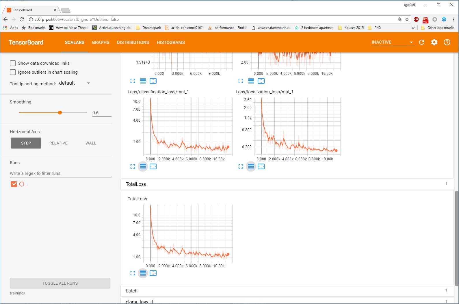
Once this is done, go to your browser and type http://localhost:6006/ in your address bar,
following which you should be presented with a dashboard similar to the one shown below
(maybe less populated if your model has just started training):
Exporting a Trained Model
Once your training job is complete, you need to extract the newly trained inference graph, which will be later used to perform the object detection. This can be done as follows:
Copy the
TensorFlow/models/research/object_detection/exporter_main_v2.pyscript and paste it straight into yourtraining_demofolder.Now, open a Terminal,
cdinside yourtraining_demofolder, and run the following command:
python .\exporter_main_v2.py --input_type image_tensor --pipeline_config_path .\models\my_ssd_resnet50_v1_fpn\pipeline.config --trained_checkpoint_dir .\models\my_ssd_resnet50_v1_fpn\ --output_directory .\exported-models\my_model
After the above process has completed, you should find a new folder my_model under the
training_demo/exported-models, that has the following structure:
training_demo/
├─ ...
├─ exported-models/
│  └─ my_model/
│     ├─ checkpoint/
│     ├─ saved_model/
│     └─ pipeline.config
└─ ...
This model can then be used to perform inference.
Note
You may get the following error when trying to export your model:
Traceback (most recent call last):
  File ".\exporter_main_v2.py", line 126, in <module>
    app.run(main)
  File "C:\Users\sglvladi\Anaconda3\envs\tf2\lib\site-packages\absl\app.py", line 299, in run
    _run_main(main, args)
  ...
  File "C:\Users\sglvladi\Anaconda3\envs\tf2\lib\site-packages\tensorflow\python\keras\engine\base_layer.py", line 1627, in get_losses_for
    reachable = tf_utils.get_reachable_from_inputs(inputs, losses)
  File "C:\Users\sglvladi\Anaconda3\envs\tf2\lib\site-packages\tensorflow\python\keras\utils\tf_utils.py", line 140, in get_reachable_from_inputs
    raise TypeError('Expected Operation, Variable, or Tensor, got ' + str(x))
TypeError: Expected Operation, Variable, or Tensor, got level_5
If this happens, have a look at the “TypeError: Expected Operation, Variable, or Tensor, got level_5” issue section for a potential solution.