Training Custom Object Detector
So, up to now you should have done the following:
Installed TensorFlow, either CPU or GPU (See TensorFlow Installation)
Installed TensorFlow Models (See TensorFlow Models Installation)
Installed labelImg (See LabelImg Installation)
Now that we have done all the above, we can start doing some cool stuff. Here we will see how you can train your own object detector, and since it is not as simple as it sounds, we will have a look at:
How to organise your workspace/training files
How to prepare/annotate image datasets
How to generate tf records from such datasets
How to configure a simple training pipeline
How to train a model and monitor it’s progress
How to export the resulting model and use it to detect objects.
Preparing workspace
If you have followed the tutorial, you should by now have a folder
Tensorflow, placed under<PATH_TO_TF>(e.g.C:\Users\sglvladi\Documents), with the following directory tree:TensorFlow ├─ addons │ └── labelImg └─ models ├── official ├── research ├── samples └── tutorialsNow create a new folder under
TensorFlowand call itworkspace. It is within theworkspacethat we will store all our training set-ups. Now let’s go under workspace and create another folder namedtraining_demo. Now our directory structure should be as so:TensorFlow ├─ addons │ └─ labelImg ├─ models │ ├─ official │ ├─ research │ ├─ samples │ └─ tutorials └─ workspace └─ training_demoThe
training_demofolder shall be our training folder, which will contain all files related to our model training. It is advisable to create a separate training folder each time we wish to train a different model. The typical structure for training folders is shown below.training_demo ├─ annotations ├─ images │ ├─ test │ └─ train ├─ pre-trained-model ├─ training └─ README.md
Here’s an explanation for each of the folders/filer shown in the above tree:
annotations: This folder will be used to store all*.csvfiles and the respective TensorFlow*.recordfiles, which contain the list of annotations for our dataset images.images: This folder contains a copy of all the images in our dataset, as well as the respective*.xmlfiles produced for each one, oncelabelImgis used to annotate objects.images\train: This folder contains a copy of all images, and the respective*.xmlfiles, which will be used to train our model.images\test: This folder contains a copy of all images, and the respective*.xmlfiles, which will be used to test our model.
pre-trained-model: This folder will contain the pre-trained model of our choice, which shall be used as a starting checkpoint for our training job.training: This folder will contain the training pipeline configuration file*.config, as well as a*.pbtxtlabel map file and all files generated during the training of our model.README.md: This is an optional file which provides some general information regarding the training conditions of our model. It is not used by TensorFlow in any way, but it generally helps when you have a few training folders and/or you are revisiting a trained model after some time.
If you do not understand most of the things mentioned above, no need to worry, as we’ll see how all the files are generated further down.
Annotating images
To annotate images we will be using the labelImg package. If you haven’t installed the package yet, then have a look at LabelImg Installation.
Once you have collected all the images to be used to test your model (ideally more than 100 per class), place them inside the folder
training_demo\images.Open a new Anaconda/Command Prompt window and
cdintoTensorflow\addons\labelImg.If (as suggested in LabelImg Installation) you created a separate Conda environment for
labelImgthen go ahead and activate it by running:activate labelImg
Next go ahead and start
labelImg, pointing it to yourtraining_demo\imagesfolder.python labelImg.py ..\..\workspace\training_demo\images
A File Explorer Dialog windows should open, which points to the
training_demo\imagesfolder.Press the “Select Folder” button, to start annotating your images.
Once open, you should see a window similar to the one below:
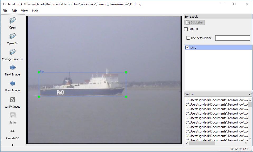
I won’t be covering a tutorial on how to use labelImg, but you can have a look at labelImg’s repo for more details. A nice Youtube video demonstrating how to use labelImg is also available here. What is important is that once you annotate all your images, a set of new *.xml files, one for each image, should be generated inside your training_demo\images folder.
Partitioning the images
Once you have finished annotating your image dataset, it is a general convention to use only part of it for training, and the rest is used for evaluation purposes (e.g. as discussed in Evaluating the Model (Optional)).
Typically, the ratio is 90%/10%, i.e. 90% of the images are used for training and the rest 10% is maintained for testing, but you can chose whatever ratio suits your needs.
Once you have decided how you will be splitting your dataset, copy all training images, together with their corresponding *.xml files, and place them inside the training_demo\images\train folder. Similarly, copy all testing images, with their *.xml files, and paste them inside training_demo\images\test.
For lazy people like myself, who cannot be bothered to do the above, I have put tugether a simple script that automates the above process:
""" usage: partition_dataset.py [-h] [-i IMAGEDIR] [-o OUTPUTDIR] [-r RATIO] [-x]

Partition dataset of images into training and testing sets

optional arguments:
  -h, --help            show this help message and exit
  -i IMAGEDIR, --imageDir IMAGEDIR
                        Path to the folder where the image dataset is stored. If not specified, the CWD will be used.
  -o OUTPUTDIR, --outputDir OUTPUTDIR
                        Path to the output folder where the train and test dirs should be created. Defaults to the same directory as IMAGEDIR.
  -r RATIO, --ratio RATIO
                        The ratio of the number of test images over the total number of images. The default is 0.1.
  -x, --xml             Set this flag if you want the xml annotation files to be processed and copied over.
"""
import os
import re
import shutil
from PIL import Image
from shutil import copyfile
import argparse
import glob
import math
import random
import xml.etree.ElementTree as ET


def iterate_dir(source, dest, ratio, copy_xml):
    source = source.replace('\\', '/')
    dest = dest.replace('\\', '/')
    train_dir = os.path.join(dest, 'train')
    test_dir = os.path.join(dest, 'test')

    if not os.path.exists(train_dir):
        os.makedirs(train_dir)
    if not os.path.exists(test_dir):
        os.makedirs(test_dir)

    images = [f for f in os.listdir(source)
              if re.search(r'([a-zA-Z0-9\s_\\.\-\(\):])+(.jpg|.jpeg|.png)$', f)]

    num_images = len(images)
    num_test_images = math.ceil(ratio*num_images)

    for i in range(num_test_images):
        idx = random.randint(0, len(images)-1)
        filename = images[idx]
        copyfile(os.path.join(source, filename),
                 os.path.join(test_dir, filename))
        if copy_xml:
            xml_filename = os.path.splitext(filename)[0]+'.xml'
            copyfile(os.path.join(source, xml_filename),
                     os.path.join(test_dir,xml_filename))
        images.remove(images[idx])

    for filename in images:
        copyfile(os.path.join(source, filename),
                 os.path.join(train_dir, filename))
        if copy_xml:
            xml_filename = os.path.splitext(filename)[0]+'.xml'
            copyfile(os.path.join(source, xml_filename),
                     os.path.join(train_dir, xml_filename))


def main():

    # Initiate argument parser
    parser = argparse.ArgumentParser(description="Partition dataset of images into training and testing sets",
                                     formatter_class=argparse.RawTextHelpFormatter)
    parser.add_argument(
        '-i', '--imageDir',
        help='Path to the folder where the image dataset is stored. If not specified, the CWD will be used.',
        type=str,
        default=os.getcwd()
    )
    parser.add_argument(
        '-o', '--outputDir',
        help='Path to the output folder where the train and test dirs should be created. '
             'Defaults to the same directory as IMAGEDIR.',
        type=str,
        default=None
    )
    parser.add_argument(
        '-r', '--ratio',
        help='The ratio of the number of test images over the total number of images. The default is 0.1.',
        default=0.1,
        type=float)
    parser.add_argument(
        '-x', '--xml',
        help='Set this flag if you want the xml annotation files to be processed and copied over.',
        action='store_true'
    )
    args = parser.parse_args()

    if args.outputDir is None:
        args.outputDir = args.imageDir

    # Now we are ready to start the iteration
    iterate_dir(args.imageDir, args.outputDir, args.ratio, args.xml)


if __name__ == '__main__':
    main()
To use the script, simply copy and paste the code above in a script named partition_dataset.py. Then, assuming you have all your images and *.xml files inside training_demo\images, just run the following command:
python partition_dataser.py -x -i training_demo\images -r 0.1
Once the script has finished, there should exist two new folders under training_demo\images, namely training_demo\images\train and training_demo\images\test, containing 90% and 10% of the images (and *.xml files), respectively. To avoid loss of any files, the script will not delete the images under training_demo\images. Once you have checked that your images have been safely copied over, you can delete the images under training_demo\images manually.
Creating Label Map
TensorFlow requires a label map, which namely maps each of the used labels to an integer values. This label map is used both by the training and detection processes.
Below I show an example label map (e.g label_map.pbtxt), assuming that our dataset containes 2 labels, dogs and cats:
item {
    id: 1
    name: 'cat'
}

item {
    id: 2
    name: 'dog'
}
Label map files have the extention .pbtxt and should be placed inside the training_demo\annotations folder.
Creating TensorFlow Records
Now that we have generated our annotations and split our dataset into the desired training and testing subsets, it is time to convert our annotations into the so called TFRecord format.
There are two steps in doing so:
Converting the individual
*.xmlfiles to a unified*.csvfile for each dataset.Converting the
*.csvfiles of each dataset to*.recordfiles (TFRecord format).
Before we proceed to describe the above steps, let’s create a directory where we can store some scripts. Under the TensorFlow folder, create a new folder TensorFlow\scripts, which we can use to store some useful scripts. To make things even tidier, let’s create a new folder TensorFlow\scripts\preprocessing, where we shall store scripts that we can use to preprocess our training inputs. Below is out TensorFlow directory tree structure, up to now:
TensorFlow
├─ addons
│   └─ labelImg
├─ models
│   ├─ official
│   ├─ research
│   ├─ samples
│   └─ tutorials
├─ scripts
│   └─ preprocessing
└─ workspace
    └─ training_demo
Converting *.xml to *.csv
To do this we can write a simple script that iterates through all *.xml files in the training_demo\images\train and training_demo\images\test folders, and generates a *.csv for each of the two.
Here is an example script that allows us to do just that:
"""
Usage:
# Create train data:
python xml_to_csv.py -i [PATH_TO_IMAGES_FOLDER]/train -o [PATH_TO_ANNOTATIONS_FOLDER]/train_labels.csv

# Create test data:
python xml_to_csv.py -i [PATH_TO_IMAGES_FOLDER]/test -o [PATH_TO_ANNOTATIONS_FOLDER]/test_labels.csv
"""

import os
import glob
import pandas as pd
import argparse
import xml.etree.ElementTree as ET


def xml_to_csv(path):
    """Iterates through all .xml files (generated by labelImg) in a given directory and combines them in a single Pandas datagrame.

    Parameters:
    ----------
    path : {str}
        The path containing the .xml files
    Returns
    -------
    Pandas DataFrame
        The produced dataframe
    """

    xml_list = []
    for xml_file in glob.glob(path + '/*.xml'):
        tree = ET.parse(xml_file)
        root = tree.getroot()
        for member in root.findall('object'):
            value = (root.find('filename').text,
                    int(root.find('size')[0].text),
                    int(root.find('size')[1].text),
                    member[0].text,
                    int(member[4][0].text),
                    int(member[4][1].text),
                    int(member[4][2].text),
                    int(member[4][3].text)
                    )
            xml_list.append(value)
    column_name = ['filename', 'width', 'height',
                'class', 'xmin', 'ymin', 'xmax', 'ymax']
    xml_df = pd.DataFrame(xml_list, columns=column_name)
    return xml_df


def main():
    # Initiate argument parser
    parser = argparse.ArgumentParser(
        description="Sample TensorFlow XML-to-CSV converter")
    parser.add_argument("-i",
                        "--inputDir",
                        help="Path to the folder where the input .xml files are stored",
                        type=str)
    parser.add_argument("-o",
                        "--outputFile",
                        help="Name of output .csv file (including path)", type=str)
    args = parser.parse_args()

    if(args.inputDir is None):
        args.inputDir = os.getcwd()
    if(args.outputFile is None):
        args.outputFile = args.inputDir + "/labels.csv"

    assert(os.path.isdir(args.inputDir))

    xml_df = xml_to_csv(args.inputDir)
    xml_df.to_csv(
        args.outputFile, index=None)
    print('Successfully converted xml to csv.')


if __name__ == '__main__':
    main()
Create a new file with name
xml_to_csv.pyunderTensorFlow\scripts\preprocessing, open it, paste the above code inside it and save.Install the
pandaspackage:conda install pandas # Anaconda # or pip install pandas # pip
Finally,
cdintoTensorFlow\scripts\preprocessingand run:# Create train data: python xml_to_csv.py -i [PATH_TO_IMAGES_FOLDER]/train -o [PATH_TO_ANNOTATIONS_FOLDER]/train_labels.csv # Create test data: python xml_to_csv.py -i [PATH_TO_IMAGES_FOLDER]/test -o [PATH_TO_ANNOTATIONS_FOLDER]/test_labels.csv # For example # python xml_to_csv.py -i C:\Users\sglvladi\Documents\TensorFlow\workspace\training_demo\images\train -o C:\Users\sglvladi\Documents\TensorFlow\workspace\training_demo\annotations\train_labels.csv # python xml_to_csv.py -i C:\Users\sglvladi\Documents\TensorFlow\workspace\training_demo\images\test -o C:\Users\sglvladi\Documents\TensorFlow\workspace\training_demo\annotations\test_labels.csv
Once the above is done, there should be 2 new files under the training_demo\annotations folder, named test_labels.csv and train_labels.csv, respectively.
Converting from *.csv to *.record
Now that we have obtained our *.csv annotation files, we will need to convert them into TFRecords. Below is an example script that allows us to do just that:
"""
Usage:

# Create train data:
python generate_tfrecord.py --label=<LABEL> --csv_input=<PATH_TO_ANNOTATIONS_FOLDER>/train_labels.csv  --output_path=<PATH_TO_ANNOTATIONS_FOLDER>/train.record

# Create test data:
python generate_tfrecord.py --label=<LABEL> --csv_input=<PATH_TO_ANNOTATIONS_FOLDER>/test_labels.csv  --output_path=<PATH_TO_ANNOTATIONS_FOLDER>/test.record
"""

from __future__ import division
from __future__ import print_function
from __future__ import absolute_import

import os
import io
import pandas as pd
import tensorflow as tf
import sys
sys.path.append("../../models/research")

from PIL import Image
from object_detection.utils import dataset_util
from collections import namedtuple, OrderedDict

flags = tf.app.flags
flags.DEFINE_string('csv_input', '', 'Path to the CSV input')
flags.DEFINE_string('output_path', '', 'Path to output TFRecord')
flags.DEFINE_string('label', '', 'Name of class label')
# if your image has more labels input them as
# flags.DEFINE_string('label0', '', 'Name of class[0] label')
# flags.DEFINE_string('label1', '', 'Name of class[1] label')
# and so on.
flags.DEFINE_string('img_path', '', 'Path to images')
FLAGS = flags.FLAGS


# TO-DO replace this with label map
# for multiple labels add more else if statements
def class_text_to_int(row_label):
    if row_label == FLAGS.label:  # 'ship':
        return 1
    # comment upper if statement and uncomment these statements for multiple labelling
    # if row_label == FLAGS.label0:
    #   return 1
    # elif row_label == FLAGS.label1:
    #   return 0
    else:
        None


def split(df, group):
    data = namedtuple('data', ['filename', 'object'])
    gb = df.groupby(group)
    return [data(filename, gb.get_group(x)) for filename, x in zip(gb.groups.keys(), gb.groups)]


def create_tf_example(group, path):
    with tf.gfile.GFile(os.path.join(path, '{}'.format(group.filename)), 'rb') as fid:
        encoded_jpg = fid.read()
    encoded_jpg_io = io.BytesIO(encoded_jpg)
    image = Image.open(encoded_jpg_io)
    width, height = image.size

    filename = group.filename.encode('utf8')
    image_format = b'jpg'
    # check if the image format is matching with your images.
    xmins = []
    xmaxs = []
    ymins = []
    ymaxs = []
    classes_text = []
    classes = []

    for index, row in group.object.iterrows():
        xmins.append(row['xmin'] / width)
        xmaxs.append(row['xmax'] / width)
        ymins.append(row['ymin'] / height)
        ymaxs.append(row['ymax'] / height)
        classes_text.append(row['class'].encode('utf8'))
        classes.append(class_text_to_int(row['class']))

    tf_example = tf.train.Example(features=tf.train.Features(feature={
        'image/height': dataset_util.int64_feature(height),
        'image/width': dataset_util.int64_feature(width),
        'image/filename': dataset_util.bytes_feature(filename),
        'image/source_id': dataset_util.bytes_feature(filename),
        'image/encoded': dataset_util.bytes_feature(encoded_jpg),
        'image/format': dataset_util.bytes_feature(image_format),
        'image/object/bbox/xmin': dataset_util.float_list_feature(xmins),
        'image/object/bbox/xmax': dataset_util.float_list_feature(xmaxs),
        'image/object/bbox/ymin': dataset_util.float_list_feature(ymins),
        'image/object/bbox/ymax': dataset_util.float_list_feature(ymaxs),
        'image/object/class/text': dataset_util.bytes_list_feature(classes_text),
        'image/object/class/label': dataset_util.int64_list_feature(classes),
    }))
    return tf_example


def main(_):
    writer = tf.python_io.TFRecordWriter(FLAGS.output_path)
    path = os.path.join(os.getcwd(), FLAGS.img_path)
    examples = pd.read_csv(FLAGS.csv_input)
    grouped = split(examples, 'filename')
    for group in grouped:
        tf_example = create_tf_example(group, path)
        writer.write(tf_example.SerializeToString())

    writer.close()
    output_path = os.path.join(os.getcwd(), FLAGS.output_path)
    print('Successfully created the TFRecords: {}'.format(output_path))


if __name__ == '__main__':
    tf.app.run()
Create a new file with name
generate_tfrecord.pyunderTensorFlow\scripts\preprocessing, open it, paste the above code inside it and save.Once this is done,
cdintoTensorFlow\scripts\preprocessingand run:# Create train data: python generate_tfrecord.py --label=<LABEL> --csv_input=<PATH_TO_ANNOTATIONS_FOLDER>/train_labels.csv --img_path=<PATH_TO_IMAGES_FOLDER>/train --output_path=<PATH_TO_ANNOTATIONS_FOLDER>/train.record # Create test data: python generate_tfrecord.py --label=<LABEL> --csv_input=<PATH_TO_ANNOTATIONS_FOLDER>/test_labels.csv --img_path=<PATH_TO_IMAGES_FOLDER>/test --output_path=<PATH_TO_ANNOTATIONS_FOLDER>/test.record # For example # python generate_tfrecord.py --label=ship --csv_input=C:\Users\sglvladi\Documents\TensorFlow\workspace\training_demo\annotations\train_labels.csv --output_path=C:\Users\sglvladi\Documents\TensorFlow\workspace\training_demo\annotations\train.record --img_path=C:\Users\sglvladi\Documents\TensorFlow\workspace\training_demo\images\train # python generate_tfrecord.py --label=ship --csv_input=C:\Users\sglvladi\Documents\TensorFlow\workspace\training_demo\annotations\test_labels.csv --output_path=C:\Users\sglvladi\Documents\TensorFlow\workspace\training_demo\annotations\test.record --img_path=C:\Users\sglvladi\Documents\TensorFlow\workspace\training_demo\images\test
Once the above is done, there should be 2 new files under the training_demo\annotations folder, named test.record and train.record, respectively.
Configuring a Training Pipeline
For the purposes of this tutorial we will not be creating a training job from the scratch, but rather we will go through how to reuse one of the pre-trained models provided by TensorFlow. If you would like to train an entirely new model, you can have a look at TensorFlow’s tutorial.
The model we shall be using in our examples is the ssd_inception_v2_coco model, since it provides a relatively good trade-off between performance and speed, however there are a number of other models you can use, all of which are listed in TensorFlow’s detection model zoo. More information about the detection performance, as well as reference times of execution, for each of the available pre-trained models can be found here.
First of all, we need to get ourselves the sample pipeline configuration file for the specific model we wish to re-train. You can find the specific file for the model of your choice here. In our case, since we shall be using the ssd_inception_v2_coco model, we shall be downloading the corresponding ssd_inception_v2_coco.config file.
Apart from the configuration file, we also need to download the latest pre-trained NN for the model we wish to use. This can be done by simply clicking on the name of the desired model in the tables found in TensorFlow’s detection model zoo. Clicking on the name of your model should initiate a download for a *.tar.gz file.
Once the *.tar.gz file has been downloaded, open it using a decompression program of your choice (e.g. 7zip, WinZIP, etc.). Next, open the folder that you see when the compressed folder is opened (typically it will have the same name as the compressed folded, without the *.tar.gz extension), and extract it’s contents inside the folder training_demo\pre-trained-model.
Now that we have downloaded and extracted our pre-trained model, let’s have a look at the changes that we shall need to apply to the downloaded *.config file (highlighted in yellow):
1 2 3 4 5 6 7 8 9 10 11 12 13 14 15 16 17 18 19 20 21 22 23 24 25 26 27 28 29 30 31 32 33 34 35 36 37 38 39 40 41 42 43 44 45 46 47 48 49 50 51 52 53 54 55 56 57 58 59 60 61 62 63 64 65 66 67 68 69 70 71 72 73 74 75 76 77 78 79 80 81 82 83 84 85 86 87 88 89 90 91 92 93 94 95 96 97 98 99 100 101 102 103 104 105 106 107 108 109 110 111 112 113 114 115 116 117 118 119 120 121 122 123 124 125 126 127 128 129 130 131 132 133 134 135 136 137 138 139 140 141 142 143 144 145 146 147 148 149 150 151 152 153 154 155 156 157 158 159 160 161 162 163 164 165 166 167 168 169 170 171 172 173 174 175 176 177 178 179 180 181 182 183 184 185 186 187 188 189 190 191 192 193 194 | # SSD with Inception v2 configuration for MSCOCO Dataset.
# Users should configure the fine_tune_checkpoint field in the train config as
# well as the label_map_path and input_path fields in the train_input_reader and
# eval_input_reader. Search for "PATH_TO_BE_CONFIGURED" to find the fields that
# should be configured.
model {
ssd {
num_classes: 1 # Set this to the number of different label classes
box_coder {
faster_rcnn_box_coder {
y_scale: 10.0
x_scale: 10.0
height_scale: 5.0
width_scale: 5.0
}
}
matcher {
argmax_matcher {
matched_threshold: 0.5
unmatched_threshold: 0.5
ignore_thresholds: false
negatives_lower_than_unmatched: true
force_match_for_each_row: true
}
}
similarity_calculator {
iou_similarity {
}
}
anchor_generator {
ssd_anchor_generator {
num_layers: 6
min_scale: 0.2
max_scale: 0.95
aspect_ratios: 1.0
aspect_ratios: 2.0
aspect_ratios: 0.5
aspect_ratios: 3.0
aspect_ratios: 0.3333
reduce_boxes_in_lowest_layer: true
}
}
image_resizer {
fixed_shape_resizer {
height: 300
width: 300
}
}
box_predictor {
convolutional_box_predictor {
min_depth: 0
max_depth: 0
num_layers_before_predictor: 0
use_dropout: false
dropout_keep_probability: 0.8
kernel_size: 3
box_code_size: 4
apply_sigmoid_to_scores: false
conv_hyperparams {
activation: RELU_6,
regularizer {
l2_regularizer {
weight: 0.00004
}
}
initializer {
truncated_normal_initializer {
stddev: 0.03
mean: 0.0
}
}
}
}
}
feature_extractor {
type: 'ssd_inception_v2' # Set to the name of your chosen pre-trained model
min_depth: 16
depth_multiplier: 1.0
conv_hyperparams {
activation: RELU_6,
regularizer {
l2_regularizer {
weight: 0.00004
}
}
initializer {
truncated_normal_initializer {
stddev: 0.03
mean: 0.0
}
}
batch_norm {
train: true,
scale: true,
center: true,
decay: 0.9997,
epsilon: 0.001,
}
}
override_base_feature_extractor_hyperparams: true
}
loss {
classification_loss {
weighted_sigmoid {
}
}
localization_loss {
weighted_smooth_l1 {
}
}
hard_example_miner {
num_hard_examples: 3000
iou_threshold: 0.99
loss_type: CLASSIFICATION
max_negatives_per_positive: 3
min_negatives_per_image: 0
}
classification_weight: 1.0
localization_weight: 1.0
}
normalize_loss_by_num_matches: true
post_processing {
batch_non_max_suppression {
score_threshold: 1e-8
iou_threshold: 0.6
max_detections_per_class: 100
max_total_detections: 100
}
score_converter: SIGMOID
}
}
}
train_config: {
batch_size: 12 # Increase/Decrease this value depending on the available memory (Higher values require more memory and vice-versa)
optimizer {
rms_prop_optimizer: {
learning_rate: {
exponential_decay_learning_rate {
initial_learning_rate: 0.004
decay_steps: 800720
decay_factor: 0.95
}
}
momentum_optimizer_value: 0.9
decay: 0.9
epsilon: 1.0
}
}
fine_tune_checkpoint: "pre-trained-model/model.ckpt" # Path to extracted files of pre-trained model
from_detection_checkpoint: true
# Note: The below line limits the training process to 200K steps, which we
# empirically found to be sufficient enough to train the pets dataset. This
# effectively bypasses the learning rate schedule (the learning rate will
# never decay). Remove the below line to train indefinitely.
num_steps: 200000
data_augmentation_options {
random_horizontal_flip {
}
}
data_augmentation_options {
ssd_random_crop {
}
}
}
train_input_reader: {
tf_record_input_reader {
input_path: "annotations/train.record" # Path to training TFRecord file
}
label_map_path: "annotations/label_map.pbtxt" # Path to label map file
}
eval_config: {
# (Optional): Uncomment the line below if you installed the Coco evaluation tools
# and you want to also run evaluation
# metrics_set: "coco_detection_metrics"
# (Optional): Set this to the number of images in your <PATH_TO_IMAGES_FOLDER>/train
# if you want to also run evaluation
num_examples: 8000
# Note: The below line limits the evaluation process to 10 evaluations.
# Remove the below line to evaluate indefinitely.
max_evals: 10
}
eval_input_reader: {
tf_record_input_reader {
input_path: "annotations/test.record" # Path to testing TFRecord
}
label_map_path: "annotations/label_map.pbtxt" # Path to label map file
shuffle: false
num_readers: 1
}
|
It is worth noting here that the changes to lines 178 and 181 above are optional. These should only be used if you installed the COCO evaluation tools, as outlined in the COCO API installation (Optional) section, and you intend to run evaluation (see Evaluating the Model (Optional)).
Once the above changes have been applied to our config file, go ahead and save it under training_demo/training.
Training the Model
Note
This tab describes the training process using Tensorflow’s new model training script, namely model_main.py, as suggested by the Tensorflow Object Detection docs. The advantage of using this script is that it interleaves training and evaluation, essentially combining the train.py and eval.py Legacy scripts.
If instead you would like to use the legacy train.py script, switch to the Legacy tab.
Before we begin training our model, let’s go and copy the TensorFlow/models/research/object_detection/model_main.py script and paste it straight into our training_demo folder. We will need this script in order to train our model.
Now, to initiate a new training job, cd inside the training_demo folder and type the following:
python model_main.py --alsologtostderr --model_dir=training/ --pipeline_config_path=training/ssd_inception_v2_coco.config
Once the training process has been initiated, you should see a series of print outs similar to the one below (plus/minus some warnings):
INFO:tensorflow:depth of additional conv before box predictor: 0
INFO:tensorflow:depth of additional conv before box predictor: 0
INFO:tensorflow:depth of additional conv before box predictor: 0
INFO:tensorflow:depth of additional conv before box predictor: 0
INFO:tensorflow:depth of additional conv before box predictor: 0
INFO:tensorflow:depth of additional conv before box predictor: 0
INFO:tensorflow:Restoring parameters from ssd_inception_v2_coco_2017_11_17/model.ckpt
INFO:tensorflow:Running local_init_op.
INFO:tensorflow:Done running local_init_op.
INFO:tensorflow:Saving checkpoints for 0 into training\model.ckpt.
INFO:tensorflow:loss = 16.100115, step = 0
...
Important
The output will normally look like it has “frozen” after the loss for step 0 has been logged, but DO NOT rush to cancel the process. The training outputs logs only every 100 steps by default, therefore if you wait for a while, you should see a log for the loss at step 100.
The time you should wait can vary greatly, depending on whether you are using a GPU and the chosen value for batch_size in the config file, so be patient.
Before we begin training our model, let’s go and copy the TensorFlow/models/research/object_detection/legacy/train.py script and paste it straight into our training_demo folder. We will need this script in order to train our model.
Now, to initiate a new training job, cd inside the training_demo folder and type the following:
python train.py --logtostderr --train_dir=training/ --pipeline_config_path=training/ssd_inception_v2_coco.config
Once the training process has been initiated, you should see a series of print outs similar to the one below (plus/minus some warnings):
INFO:tensorflow:depth of additional conv before box predictor: 0
INFO:tensorflow:depth of additional conv before box predictor: 0
INFO:tensorflow:depth of additional conv before box predictor: 0
INFO:tensorflow:depth of additional conv before box predictor: 0
INFO:tensorflow:depth of additional conv before box predictor: 0
INFO:tensorflow:depth of additional conv before box predictor: 0
INFO:tensorflow:Restoring parameters from ssd_inception_v2_coco_2017_11_17/model.ckpt
INFO:tensorflow:Running local_init_op.
INFO:tensorflow:Done running local_init_op.
INFO:tensorflow:Starting Session.
INFO:tensorflow:Saving checkpoint to path training\model.ckpt
INFO:tensorflow:Starting Queues.
INFO:tensorflow:global_step/sec: 0
INFO:tensorflow:global step 1: loss = 13.8886 (12.339 sec/step)
INFO:tensorflow:global step 2: loss = 16.2202 (0.937 sec/step)
INFO:tensorflow:global step 3: loss = 13.7876 (0.904 sec/step)
INFO:tensorflow:global step 4: loss = 12.9230 (0.894 sec/step)
INFO:tensorflow:global step 5: loss = 12.7497 (0.922 sec/step)
INFO:tensorflow:global step 6: loss = 11.7563 (0.936 sec/step)
INFO:tensorflow:global step 7: loss = 11.7245 (0.910 sec/step)
INFO:tensorflow:global step 8: loss = 10.7993 (0.916 sec/step)
INFO:tensorflow:global step 9: loss = 9.1277 (0.890 sec/step)
INFO:tensorflow:global step 10: loss = 9.3972 (0.919 sec/step)
INFO:tensorflow:global step 11: loss = 9.9487 (0.897 sec/step)
INFO:tensorflow:global step 12: loss = 8.7954 (0.884 sec/step)
INFO:tensorflow:global step 13: loss = 7.4329 (0.906 sec/step)
INFO:tensorflow:global step 14: loss = 7.8270 (0.897 sec/step)
INFO:tensorflow:global step 15: loss = 6.4877 (0.894 sec/step)
...
If you ARE observing a similar output to the above, then CONGRATULATIONS, you have successfully started your first training job. Now you may very well treat yourself to a cold beer, as waiting on the training to finish is likely to take a while. Following what people have said online, it seems that it is advisable to allow you model to reach a TotalLoss of at least 2 (ideally 1 and lower) if you want to achieve “fair” detection results. Obviously, lower TotalLoss is better, however very low TotalLoss should be avoided, as the model may end up overfitting the dataset, meaning that it will perform poorly when applied to images outside the dataset. To monitor TotalLoss, as well as a number of other metrics, while your model is training, have a look at Monitor Training Job Progress using TensorBoard.
If you ARE NOT seeing a print-out similar to that shown above, and/or the training job crashes after a few seconds, then have a look at the issues and proposed solutions, under the Common issues section, to see if you can find a solution. Alternatively, you can try the issues section of the official Tensorflow Models repo.
Note
Training times can be affected by a number of factors such as:
The computational power of you hardware (either CPU or GPU): Obviously, the more powerful your PC is, the faster the training process.
Whether you are using the TensorFlow CPU or GPU variant: In general, even when compared to the best CPUs, almost any GPU graphics card will yield much faster training and detection speeds. As a matter of fact, when I first started I was running TensorFlow on my Intel i7-5930k (6/12 cores @ 4GHz, 32GB RAM) and was getting step times of around 12 sec/step, after which I installed TensorFlow GPU and training the very same model -using the same dataset and config files- on a EVGA GTX-770 (1536 CUDA-cores @ 1GHz, 2GB VRAM) I was down to 0.9 sec/step!!! A 12-fold increase in speed, using a “low/mid-end” graphics card, when compared to a “mid/high-end” CPU.
How big the dataset is: The higher the number of images in your dataset, the longer it will take for the model to reach satisfactory levels of detection performance.
The complexity of the objects you are trying to detect: Obviously, if your objective is to track a black ball over a white background, the model will converge to satisfactory levels of detection pretty quickly. If on the other hand, for example, you wish to detect ships in ports, using Pan-Tilt-Zoom cameras, then training will be a much more challenging and time-consuming process, due to the high variability of the shape and size of ships, combined with a highly dynamic background.
And many, many, many, more….
Evaluating the Model (Optional)
By default, the training process logs some basic measures of training performance. These seem to change depending on the installed version of Tensorflow and the script used for training (i.e. model_main.py (Standard) or train.py (Legacy)).
As you will have seen in various parts of this tutorial, we have mentioned a few times the optional utilisation of the COCO evaluation metrics. Also, under section _image_partitioning_sec we partitioned our dataset in two parts, where one was to be used for training and the other for evaluation. In this section we will look at how we can use these metrics, along with the test images, to get a sense of the performance achieved by our model as it is being trained.
Firstly, let’s start with a brief explanation of what the evaluation process does. While the training process runs, it will occasionally create checkpoint files inside the training_demo/training folder, which correspond to snapshots of the model at given steps. When a set of such new checkpoint files is generated, the evaluation process uses these files and evaluates how well the model performs in detecting objects in the test dataset. The results of this evaluation are summarised in the form of some metrics, which can be examined over time.
The steps to run the evaluation are outlined below:
Firstly we need to download and install the metrics we want to use.
For a description of the supported object detection evaluation metrics, see here.
The process of installing the COCO evaluation metrics is described in COCO API installation (Optional).
Secondly, we must modify the configuration pipeline (
*.configscript).
See lines 178 and 181 of the script in Configuring a Training Pipeline.
The third step depends on what method (script) was used when staring the training in Training the Model. See below for details:
The
model_main.pyscript interleaves training and evaluation. Therefore, assuming that the following two steps were followed correctly, nothing else needs to be done.When using the Legacy scripts, evaluation is run using the
eval.pyscript. This is done as follows:Copy the
TensorFlow/models/research/object_detection/legacy/eval.pyscript and paste it inside thetraining_demofolder.Now, to initiate an evaluation job,
cdinside thetraining_demofolder and type the following:python eval.py --logtostderr --pipeline_config_path=training/ssd_inception_v2_coco.config --checkpoint_dir=training/ --eval_dir=training/eval_0
While the evaluation process is running, it will periodically (every 300 sec by default) check and use the latest training/model.ckpt-* checkpoint files to evaluate the performance of the model. The results are stored in the form of tf event files (events.out.tfevents.*) inside training/eval_0. These files can then be used to monitor the computed metrics, using the process described by the next section.
Monitor Training Job Progress using TensorBoard
A very nice feature of TensorFlow, is that it allows you to coninuously monitor and visualise a number of different training/evaluation metrics, while your model is being trained. The specific tool that allows us to do all that is Tensorboard.
To start a new TensorBoard server, we follow the following steps:
Open a new Anaconda/Command Prompt
Activate your TensorFlow conda environment (if you have one), e.g.:
activate tensorflow_gpu
cdinto thetraining_demofolder.Run the following command:
tensorboard --logdir=training\
The above command will start a new TensorBoard server, which (by default) listens to port 6006 of your machine. Assuming that everything went well, you should see a print-out similar to the one below (plus/minus some warnings):
TensorBoard 1.6.0 at http://YOUR-PC:6006 (Press CTRL+C to quit)
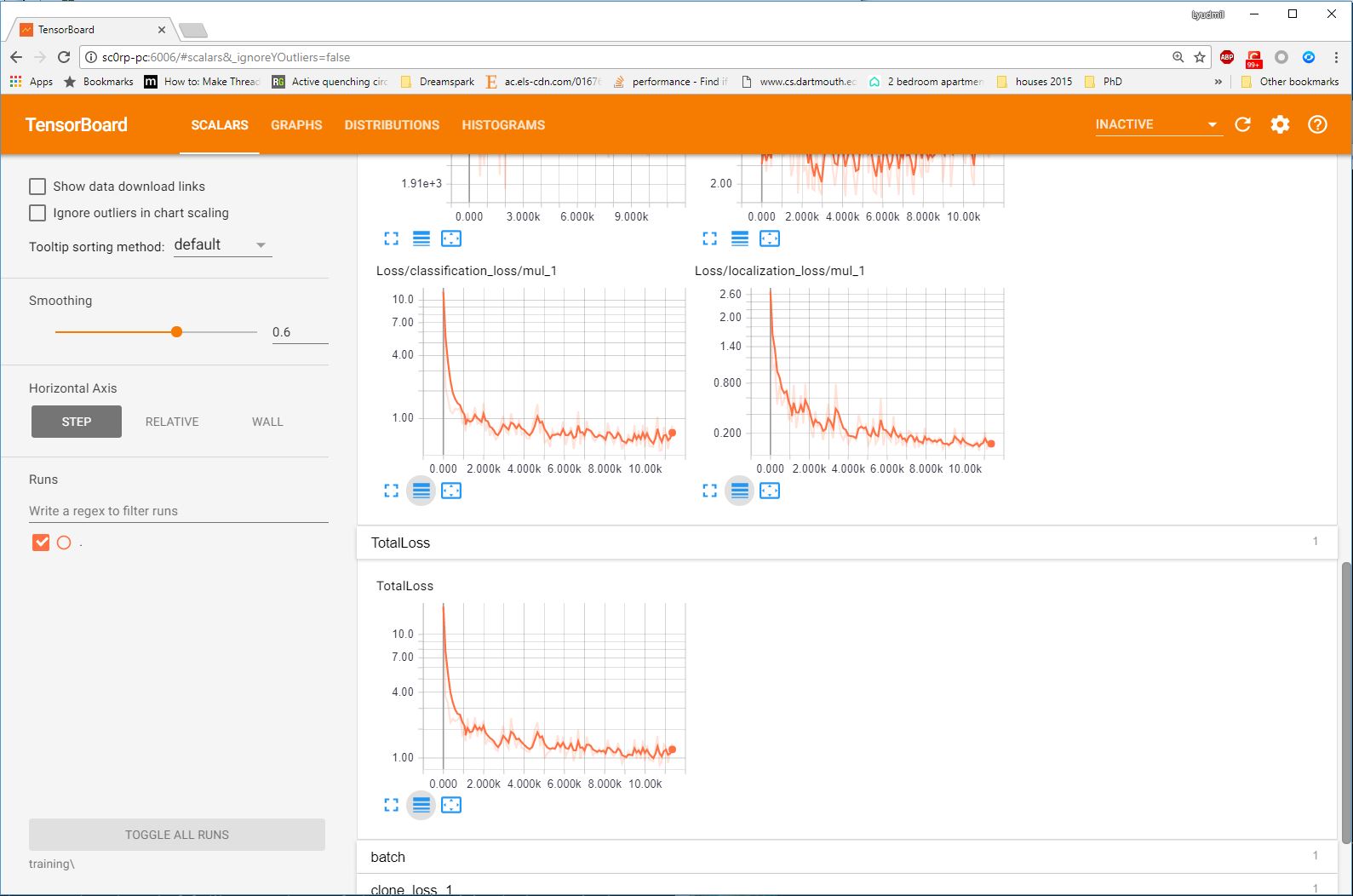
Once this is done, go to your browser and type http://YOUR-PC:6006 in your address bar, following which you should be presented with a dashboard similar to the one shown below (maybe less populated if your model has just started training):
Exporting a Trained Inference Graph
Once your training job is complete, you need to extract the newly trained inference graph, which will be later used to perform the object detection. This can be done as follows:
Open a new Anaconda/Command Prompt
Activate your TensorFlow conda environment (if you have one), e.g.:
activate tensorflow_gpu
Copy the
TensorFlow/models/research/object_detection/export_inference_graph.pyscript and paste it straight into yourtraining_demofolder.Check inside your
training_demo/trainingfolder for themodel.ckpt-*checkpoint file with the highest number following the name of the dash e.g.model.ckpt-34350). This number represents the training step index at which the file was created.Alternatively, simply sort all the files inside
training_demo/trainingby descending time and pick themodel.ckpt-*file that comes first in the list.Make a note of the file’s name, as it will be passed as an argument when we call the
export_inference_graph.pyscript.Now,
cdinside yourtraining_demofolder, and run the following command:
python export_inference_graph.py --input_type image_tensor --pipeline_config_path training/ssd_inception_v2_coco.config --trained_checkpoint_prefix training/model.ckpt-13302 --output_directory trained-inference-graphs/output_inference_graph_v1.pb